Model evaluation is very important stage of a machine learning pipeline to understand the robustness. Herein, ROC Curves and AUC score are one of the most common evaluation techniques for multiclass classification problems based on neural networks, logistic regression or gradient boosting. In this post, we are going to explain ROC Curves and AUC score, and also we will mention why we need those explainers in a timeline.

Vlog
ROC Curves and AUC are mentioned in the following video. You can either watch the following video or follow this blog post. They both cover those evaluation techniques.
🙋♂️ You may consider to enroll my top-rated machine learning course on Udemy

Accuracy is not enough
Accuracy is not enough to evaluate a machine learning model. Consider fraud detection or cancer diagnosis cases. Just a few of instances are true in those cases. If your program returns not fraud or not cancer by default, then your classifier would have a high accuracy score.
def classifier(X):
   #ignore input X features
   return False
But the important thing is here to find those rare events. That’s why, we mostly evaluate classification cases with precision and recall score.

Precision is sometimes not enough
If you have distinct prediction classes, then it is easy to calculate precision and recall. For example, regular decision tree algorithms such as ID3 or C4.5 predict custom classes nominally.
But sometimes it’s not that easy. Some algorithms neural networks, logistic regression and gradient boosting predict continuous scores instead of custom classes.
A case study
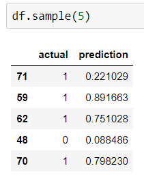
Let’s see why single precision and recall scores are sometimes not enough in a hands on case. We are going to read the following data set. It stores actual classes and prediction scores of 100 instances. Actual column stores 0 and 1 classes and they are half half balanced. Prediction column stores the probability scores in scale of [0, 1].
import pandas as pd
#Ref: https://github.com/serengil/tensorflow-101/blob/master/dataset/auc-case-predictions.csv
df = pd.read_csv("auc-case-predictions.csv")
Scores to custom classes
Here, it is expected that classify some predictions to 1 and some others to 0. The easiest way to do this is to check its value is greater than a threshold value. For example, let’s set the threshold to 0.5. I’m going to count confusion matrix items for this threshold.
threshold = 0.5
tp = 0; fp = 0; fn = 0; tn = 0
Now, I’m going to classify a prediction to 1 if it is greater than the threshold value.
for index, instance in df.iterrows():
   actual = instance["actual"]
   prediction = instance["prediction"]

   if prediction >= threshold:
      prediction_class = 1
   else:
      prediction_class = 0
Now, it is easy to find the precision and recall if you have custom predictions. But we need to find confusion matrix first.
if prediction_class == 1 and actual == 1:
   tp = tp + 1
elif actual == 1 and prediction_class == 0:
   fn = fn + 1
elif actual == 0 and prediction_class == 1:
   fp = fp + 1
elif actual == 0 and prediction_class == 0:
   tn = tn + 1
Then, we will calculate the true positive rates and false positive rates when we counted the confusion matrix items.
tpr = tp / (tp + fn)
fpr = fp / (tn + fp)
True positive rate is 0.74 and false positive rate is 0.24 when the threshold value is 0.5. The question is that could I have a higher scores for a different threshold value? ROC curve exactly examines this question.
Tuning the threshold
Notice that actual classes are 0 and 1; prediction scores are in scale of [0, 1]. So, threshold value could be change in scale of [0, 1] as well. I can start from 0, and increase the step size 0.001 until threshold becomes 1 as shown below. Thus, we will calculate true positive rate and false positive rate for each 1000 different threshold values.
import numpy as np

roc_point = []
thresholds = list(np.array(list(range(0, 1000+1, 1)))/1000)

for threshold in thresholds:
   #do tpr and fpr calculations in this for loop.
   #...
   roc_point.append([tpr, fpr])
Then, it would be easy to store true positive and false positive rates for each threshold value in a pandas data frame.
pivot = pd.DataFrame(roc_point, columns = ["x", "y"])
pivot["threshold"] = thresholds

ROC Curve
I’m going to plot a scatter. X-axis value will be false positive rate whereas Y-axis value will be true positive rate for each threshold.
plt.scatter(pivot.y, pivot.x)
plt.plot([0, 1])
plt.xlabel('false positive rate')
plt.ylabel('true positive rate')

Notice that this is a binary classification task and a random number generator would have 50% accuracy because data set is balaced. The linear line on the graph shows the accuracy of random number generator. The perfect classifier would have a inverse shape of L letter. Our prediction score has that curve. It is better than random number generator and worse than the perfect classifier.
AUC Score
AUC is the acronym of area under curve. We know that the perfect classifier would have square shape and its area becomes 1. Random number generator has a triangle shape and its area becomes 0.5. It seem s that our curve has an area greater than 0.5 and less than 1. Finding the exact area requires integral calculus but numpy luckily handles this calculation.
from numpy import trapz
auc = round(abs(np.trapz(pivot.x, pivot.y)), 4)
AUC score is 0.7918 for those predictions. However, this is an approximate value because if we increase the number of points in thresholds list, then area might change. Still, this is enough to evaluate the predictions. It has 79.18% accuracy based on AUC score.
Conclusion
So, we have mentioned ROC Curve and AUC scores, and why we need those explainers in a case study. We’ve shown those concepts for a binary classification task but multiclass classification task could be converted to n times binary classification task. In other words, it can be applied to multiclass classification tasks as well.
I pushed the source code of this study to GitHub. You can support this study if you star⭐️ the repo.
Support this blog financially if you do like!


