We’ve recently mentioned beauty score prediction. However, that study is mainly based on the study of South China University of Technology. Researchers shared a data set including beauty scores. However, beauty scores are labeled as unbiased. No Latino, Indian and Black people exist in the data set. That’s why, applying that model to independent communities causes to find White or Asian people as the most beautiful ones. Herein, The University of Chicago published a Chicago Face Database. It is a 1.24 GB zipped data set consisting of 600 people and 1200 facial photos. The data is rich. It has emotion, race, age and gender features already. I’ve built different machine learning model for those features. This data set might help those studies to improve. Interestingly, this data set also has some additional scores such as attractiveness and babyface. These score are obtained from hundreds of labelers.

An unbiased study
Chicago face database offers unbiased data set because attractiveness and babyface of people are scored with respect to other people of the same race and gender. For example, the following illustration shows attractiveness scores for different races including White, Black, Latino and Asian.
🙋♂️ You may consider to enroll my top-rated machine learning course on Udemy


Data set
Download page directs you to a request form. Download link will be shared in minutes when you complete the form. There is no supervisor to approve. You will download cfd.zip and the file “CFD 2.0.3 Norming Data and Codebook.xlsx” in the zip will guide you. I removed the lines above the header and save the file as metadata.csv to read in my python code.
cfd_df_raw = pd.read_csv("metadata.csv")
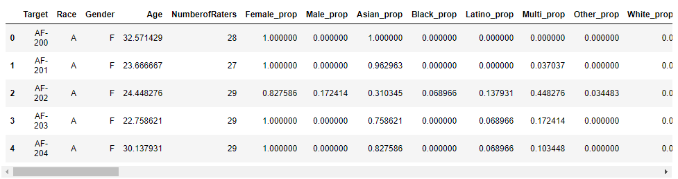
Target refers to the folder name. It also state the declared race and gender. For example, the first line means 200th Asian Female in the data set. Some folders include several images. I will append list of including file names as a column.
def getFileNames(target):
   files = []
   file_count = 0
   path = "CFD_Version_203/CFD_203_Images/%s/" % (target)
   for r, d, f in os.walk(path):
      for file in f:
         if ('.jpg' in file) or ('.jpeg' in file) or ('.png' in file):
            files.append(file)
   return files

cfd_df_raw["files"] = cfd_df_raw.Target.apply(getFileNames)

I should store each file an instance. In other words, number of rows of the data set should be equal to the number of total files. I will build two for loops. First iterates on the folder names (Target column value) and second iterates on the files. I will store this in a new data frame.
cfd_instances = []
for index, instance in cfd_df_raw.iterrows():
    folder = instance.Target
    score = instance['Attractive']
    for file in instance.files:
        tmp_instance = []
        tmp_instance.append(folder)
        tmp_instance.append(file)
        tmp_instance.append(score)
        cfd_instances.append(tmp_instance)

df = pd.DataFrame(cfd_instances, columns = ["folder", "file", "score"])
We have the exact location of the file (folder and file name) and its target score to model. We should append the pixel values of the file as a column. This will be the only feature in the modelling step.
def retrievePixels(path):
    img = image.load_img(path, grayscale=False, target_size=(224, 224))
    x = image.img_to_array(img).reshape(1, -1)[0]
    return x

df['exact_file'] = "CFD_Version_203/CFD_203_Images/"+df["folder"]+"/"+df['file']
df['pixels'] = df['exact_file'].apply(retrievePixels)
To be honest, I firstly tried to combine Chicago and South China data sets but it would not overperform. Firstly, being beautiful and being attractive are different. Secondly, data sets have different scales of scores. The one is scored in [1, 5] and the second is scored in [1, 7]. Also, they have different distributions and standard deviations. That’s why, I will build a custom model for attractiveness prediction.
To avoid manipulation
People pose for different emotion. Neutral and happy facial expressions are OK but I will discard angry and fearful expressions. Because I would like to find the most attractive actors / actresses at the end and IMDb data set has no those kind of profile photos. Including just neutral and happy expressions causes to decrease the data set size to 904. As I mentioned folder name contains emotion.
def findEmotion(file):
    #sample file name CFD-WM-040-023-HO.jpg
    file_name = file.split(".")[0] #[1] is jpg
    emotion = file_name.split("-")[4]
    return emotion

df['emotion'] = df.file.apply(findEmotion)

#include neutral, happen open mouth and happy close mouth
df = df[(df.emotion == 'N') | (df.emotion == 'HO') | (df.emotion == 'HC')]
Pre-processing
We’ve added the pixel values as a feature and we also have the target score value in the data frame. We could ignore the rest of the columns. Image pixels were stored in 1D array but VGG-Face model expects 3D array. Also, pixel values are in [0, 255] and we should normalize inputs in [0, 1].
features = []
pixels = df['pixels'].values
for i in range(0, pixels.shape[0]):
    features.append(pixels[i])

features = np.array(features)
features = features.reshape(features.shape[0], 224, 224, 3)

features = features / 255
Train test split
Splitting the data set into train, test and validation sets is a common way to avoid overfitting but we do not have a large set of data set. Total number of instances is 904. That’s why, I will just use train and validation sets to increase the number of train instances.
train_x, val_x, train_y, val_y = train_test_split(features, df.score.values, test_size=0.3, random_state=17)
VGG-Face
We will apply transfer learning and use VGG-Face model as a base model.
base_model = Sequential()
base_model.add(ZeroPadding2D((1,1),input_shape=(224,224, 3)))
base_model.add(Convolution2D(64, (3, 3), activation='relu'))
base_model.add(ZeroPadding2D((1,1)))
base_model.add(Convolution2D(64, (3, 3), activation='relu'))
base_model.add(MaxPooling2D((2,2), strides=(2,2)))

base_model.add(ZeroPadding2D((1,1)))
base_model.add(Convolution2D(128, (3, 3), activation='relu'))
base_model.add(ZeroPadding2D((1,1)))
base_model.add(Convolution2D(128, (3, 3), activation='relu'))
base_model.add(MaxPooling2D((2,2), strides=(2,2)))

base_model.add(ZeroPadding2D((1,1)))
base_model.add(Convolution2D(256, (3, 3), activation='relu'))
base_model.add(ZeroPadding2D((1,1)))
base_model.add(Convolution2D(256, (3, 3), activation='relu'))
base_model.add(ZeroPadding2D((1,1)))
base_model.add(Convolution2D(256, (3, 3), activation='relu'))
base_model.add(MaxPooling2D((2,2), strides=(2,2)))

base_model.add(ZeroPadding2D((1,1)))
base_model.add(Convolution2D(512, (3, 3), activation='relu'))
base_model.add(ZeroPadding2D((1,1)))
base_model.add(Convolution2D(512, (3, 3), activation='relu'))
base_model.add(ZeroPadding2D((1,1)))
base_model.add(Convolution2D(512, (3, 3), activation='relu'))
base_model.add(MaxPooling2D((2,2), strides=(2,2)))

base_model.add(Convolution2D(4096, (7, 7), activation='relu'))
base_model.add(Dropout(0.5))
base_model.add(Convolution2D(4096, (1, 1), activation='relu'))
base_model.add(Dropout(0.5))
base_model.add(Convolution2D(2622, (1, 1)))
base_model.add(Flatten())
base_model.add(Activation('softmax'))

#pre-trained weights of vgg-face model.
#you can find it here: https://drive.google.com/file/d/1CPSeum3HpopfomUEK1gybeuIVoeJT_Eo/view?usp=sharing
#related blog post: https://sefiks.com/2018/08/06/deep-face-recognition-with-keras/
base_model.load_weights('vgg_face_weights.h5')
This model is tuned for face recognition applications. Its early layers can detect some facial attributes. We will lock the early layers to have some outcomes. We will expect model to learn attractiveness at the final layers. Also, the base model has 2622 outputs but this application will have just one output which is attractiveness score.
num_of_classes = 1 #this is a regression problem

#freeze all layers of VGG-Face except last 7 one
for layer in base_model.layers[:-7]:
    layer.trainable = False

base_model_output = Sequential()
base_model_output = Flatten()(base_model.layers[-4].output)
base_model_output = Dense(num_of_classes)(base_model_output)

attractiveness_model = Model(inputs=base_model.input, outputs=base_model_output)
Training
This is a regression problem. That’s why, loss function should be MSE. To learn faster, I will use ADAM as a optimization algorithm. Finally, I set the epoch to a very large number but monitor loss and terminate the training if validation loss would not decrease for 50 rounds. In this way, I can avoid overfitting.
attractiveness_model.compile(loss='mean_squared_error'
, optimizer=keras.optimizers.Adam())

checkpointer = ModelCheckpoint(filepath='attractiveness.hdf5'
    , monitor = "val_loss", verbose=1
, save_best_only=True, mode = 'auto'
)

earlyStop = EarlyStopping(monitor='val_loss', patience=50)

score = attractiveness_model.fit(train_x, train_y, epochs=5000
    , validation_data=(val_x, val_y), callbacks=[checkpointer, earlyStop]
)
Loss
My experiment is terminated in 165th round because validation loss didn’t decrease for 50 rounds. Loss graphic seems to be acceptable.
best_iteration = np.argmin(score.history['val_loss'])+1
val_scores = score.history['val_loss'][0:best_iteration]
train_scores = score.history['loss'][0:best_iteration]

plt.plot(val_scores, label='val_loss')
plt.plot(train_scores, label='train_loss')
plt.legend(loc='upper right')
plt.show()

Performance
predictions = attractiveness_model.predict(val_x)
actuals = val_y

perf = pd.DataFrame(actuals, columns = ["actuals"])
perf["predictions"] = predictions

print("pearson correlation: ",perf[['actuals', 'predictions']].corr(method ='pearson').values[0,1])
print("mae: ", mean_absolute_error(actuals, predictions))
print("rmse: ", sqrt(mean_squared_error(actuals, predictions)))
I got the following error metrics. Consider that attractiveness score is in [1, 7] and we can predict it with ±0.3 error based on MAE.
pearson correlation: 0.7744527538483897
mae: 0.3489213796665445
rmse: 0.46873142978897514
Visualizing the validation set accuracy
Imagining the error metrics might be hard. That’s why, I plot predictions and actual values for validation set always.
min_limit = df.score.min(); max_limit = df.score.max()
best_predictions = []

for i in np.arange(int(min_limit), int(max_limit)+1, 0.01):
    best_predictions.append(round(i, 2))
plt.scatter(best_predictions, best_predictions, s=1, color = 'black', alpha=0.5)
plt.scatter(predictions, actuals, s=20, alpha=0.1)

Scatter plot show that predictions are the perfect but they are acceptable.
IMDb data set
We can test the built model for IMDb data set. We’ve used that data set in one of our studies. We will use the data set similarly. You should read that blog post to dive deep to this data set. The data set consists of almost 100K samples and genders are distributed uniformly in the data set. The following video slide shows the most 25 attractive actresses judged by AI. Here, you can find the full imdb list. Also, the following video slide shows the 25 most attractive ones descendingly.
Babyface score
The data set has also babyface score labels. When you set the babyface score instead of attractiveness score, then you can find the celebrities having the highest babyface score. BTW, this is parametric in the source notebook. The following video slide show the most 25 babyface actors in imdb data set.
Conclusion
So, we’ve built a machine learning model to generalize the attractiveness score based on facial photos and results seem to be acceptable. Then, we’ve tested the built model on a large IMDb data set to find the most attractive celebrities. How anyone can create his own list, these results are the consequence of perception of people majority.
I’ve pushed the source code of this study as a notebook to GitHub.
Support this blog financially if you do like!


